(lightly revised 13 July 2025, Gompertz appendix added 17 November 2025)
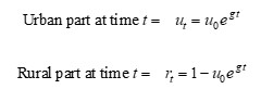
This article by the investor Claire Barnes of Apollo Investment Management highlights an interesting property of compound growth at a fixed percentage rate, in any quantity which forms part of a finite whole. In summary, the point is this. Suppose urban land area + rural land area = 1 (ie a finite land area), and assume urban land area grows at a constant percentage rate (in line with the ‘economic growth’ universally sought by governments). Then it follows that rural land area doesn’t just decline, it declines at an accelerating percentage rate.
Claire’s illustration copied below shows the case where rural land is initially 85% of the total, urban land is 15%, and urban land grows at 5% per annum. On these parameters, the rural land is extinguished after about 38 years.
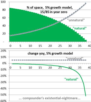
Note the alarming and invidious property of the second graph. For many years the percentage rate of decline in the rural part is very small, too small for most people to notice. Then suddenly the rate of decline speeds up and the remaining rural part disappears quickly, too quickly to do anything about it.
The accelerating rate of decline of the second part is the growth rate of the first part, scaled by the current relative size of the two parts. The intuition is that one unit of land added to the urban part must equal one unit subtracted from the rural part. So to get the percentage rate of decay in the rural part, we need to re-scale the fixed 5% in proportion to the current relative sizes of the two parts.
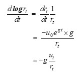
To confirm this algebraically, it is neater to work with continuously compounded rates of growth and decay, rather than annual rates. (E.g. for the 5% per annum in the example above, we use a continuously compounded rate of say g = log(1.05) = 0.0479). We then have:
The percentage rate of growth (here negative, i.e. decay) of the rural part is (d r_t / dt) divided by r_t (also equivalent to the the semi-logarithmic derivative d(log r_t) / dt). This is:
The time until the rural part is exhausted is given by setting the equation for “rural part at time t” to 0. This gives

which for u(0) = 15% and g = log(1.05) = 0.0479 gives 38.9 years, consistent with the graph above. In words: the time to extinction of the rural part is inversely proportional to the growth rate of the urban part.
Pages 12-13 of this report from the World Bank give some data on current urban land and rates of growth, which suggest that for most Asian countries, the outlook is not quite as bad as suggested by the graph above. But there are probably ambiguities with the definition and measurement of “urban” and “rural”. And whatever the exact parameters, a precautionary principle seems sensible, because the overall pattern is quite general: when one part increases at a constant percentage rate, the other part doesn’t just decline, it declines at an accelerating percentage rate.
I agree that this does not seem to be widely appreciated. Perhaps ecologists know it, but on a quick search I could not find obviously relevant commentary.
Claire suggests a couple of reasons why it may be neglected. First, individuals and governments tend to focus more on things which show compound growth, because that is where Investment and career and taxation opportunities tend to be found. We tend to be less aware of complementary things which are declining. Second, evidence-based people focus on things which are quantified; but things which are declining tend not to be quantified, precisely because of the lack of positive opportunities. I agree with both these points.
The alarming property of the graph is the “gradually, then suddenly” pattern of the rural part’s decline. The rural decline is not exponential (a constant g percentage rate of decline), it’s worse than that: it’s an accelerating percentage rate of decline.
There is a famous quote by Ernest Hemingway: “How did you go bankrupt?” — “Two ways. Gradually, then suddenly”. Perhaps we should call the pattern of a slow-then-fast percentage rate of decline a “Hemingway decay”.
We can then summarise like this:
Where two parts form a finite whole, and one part increases at a constant percentage rate, the second part declines at an acccelerating percentage rate. It declines gradually, then suddenly: Hemingway decay.
___________________________________
Geeky Gompertz appendix (17/11/25)
Actuaries may notice an analogy between the two-parts-of-a-whole urban and rural areas, and the two-possible-states in a mortality model of dead and alive. Yes: at time t, the rural part is the fraction of the land still “alive” (tp0 in actuarial notation), and the urban part is the fraction “dead” (tq0 in actuarial notation).
In this 200th anniversary year of the famous Gompertz model of mortality, I thought connections between this and Hemingway decay might be worth exploring. Spoiler: in the end the juice probably isn’t worth the squeeze. But here goes….
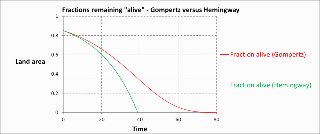
Both lines in the graph use the same 5% growth rate. The difference is in what’s growing – a state (Hemingway) or a transition rate (Gompertz):
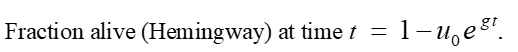
- Hemingway assumes the urban area or fraction dead grows exponentially: ut = u0 e gt. The thing that’s growing constantly is the state (i.e. dead, or urban).
- Gompertz assumes the hazard rate (rate of death) grows exponentially: ht = h0 e gt. The thing that’s growing constantly is the transition rate (i.e. from alive to dead, or rural to urban).
By standard arguments, the Gompertz fraction alive (rural area) is the exponential of minus the integrated hazard rate:
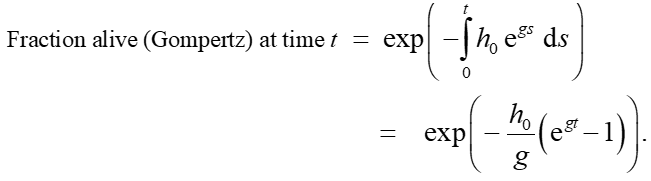
Notice that this involves an “exponential of an exponential” – a so-called tower of exponentials (e-e) – and hence the initially accelerating rate of decline in the fraction alive. In the early years, this is similar to the accelerating rate of decline in the fraction alive in the simpler Hemingway formula:
But at longer durations, the decline in the Hemingway fraction alive keeps accelerating while that in Gompertz slows down, and eventually the second derivative of the Gompertz fraction alive turns turns positive.
Algebraically, the second derivative is
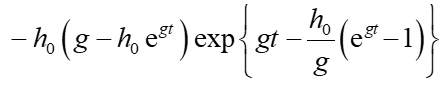
and the initial hazard rate, h0, is (roughly) h0 = 0.15 x 0.05 = 0.0075. Then solving for the time where this second derivative is zero gives t ≈ 45, consistent with the position of the inflexion point in the red line in the chart.
To summarise: Hemingway and Gompertz aren’t the same (of course they aren’t, hell-raising novelist and actuary). But in the early years, they’re close.