This blog first makes a brief comment on an interesting recent paper by Mathias Lindholm, Ronald Richman, Andreas Tsanakas and Mario Wüthrich. I then expand on two points tangential to their paper: non-risk price discrimination, which they touched on in their concluding comments by referencing a previous discussion note from me; and loss coverage, which was included in earlier drafts of that same note before its unfortunate deletion by an editor.
Perspectives on fairness
The perspective on fairness in the paper requires that there is “no relation” between predicted claims costs and banned variables. The differences between the various concepts (discrimination-free price, demographic parity, equalised odds, predictive parity) appear to be in how exactly “no relation” is defined, e.g. whether inferences made about banned variables from permitted variables constitute a “relation” between banned variables and predicted costs.
Another perspective on fairness, arguably a more limited one, is to require that prediction process has similar technical performance across all population groups. “Technical performance” is defined here by properties such as: well-calibrated for each group, equal false positive rates for each group (for prediction of “high risk”), and equal false negative rates for each group. “Well-calibrated” means that the predicted probability of loss for a group corresponds to its actual probability of loss.
To illustrate, suppose the prediction process is based on “red-lining” (blanket assignment of a “high risk” prediction to the populations of predominantly Black areas). But within the red-lined areas, there may be some lower-risk enclaves; and so for applicants from these enclaves, the assignment will be wrong (false positive for “high risk”). Since the applicants from these enclaves are predominantly Black, this false positive result is likely to affect Blacks at a higher rate than other ethnic groups. This would fail the criterion of equal false positive rates across Black versus other ethnic groups. (There are other reasons why red-lining might be considered unfair, e.g. reinforcement of pre-existing disadvantage, reinforcement of prejudice, lack of controllability, etc. Chapter 7 of my book Loss Coverage gives a taxonomy of objections to risk classification.)
This more limited and technical perspective on fairness may seem closer to “what an insurer would want to do anyway”, even absent any regulation: good performance of the prediction process equals good underwriting. But it turns out to have its own technical problems, arising from what I call the statistical fairness trilemma.
Statistical fairness trilemma
The statistical fairness trilemma, stated for binary prediction, says that where the base rates (say probability of claim) differ across the groups, a binary predictor can satisfy at most two out of the three plausible performance criteria: well-calibrated for each group, equal false positive rates for each group, and equal false negative rates for each group. (One trivial exception: a perfect predictor which classifies all cases correctly is well-calibrated with equal (zero) false positives and negatives.)
The trilemma is demonstrated for a simple example here. The appendix at the end of this blog gives an alternative presentation. The idea can be extended for non-binary predictions; indeed I sometimes get the impression, skimming recent data science papers, that they have stumbled across some version of the idea and thought it is something new.
It’s interesting that both perspectives quickly run into problems: statistical fairness leads to the above trilemma, and the group fairness axioms from machine learning may all be incompatible with the seemingly reasonable discrimination-free price. I wonder if there are any further insights available from comparing and contrasting the problems of the two perspectives. If anyone has any clearer thoughts on this, I would be interested to read about them.
What is fair v. what is effective?
Partly because of the inconclusive and somewhat arbitrary nature of any discussion of fairness, I am also interested in the question: what is effective? That is, what is most beneficial for society as a whole?
Most actuaries and economists think they already know the answer to this question: risk classification using the fullest possible information is efficient. And so (the argument goes) any restriction on risk classification involves a trade-off between social dislike of discrimination versus insurance market efficiency.
As a matter of simple arithmetic, I think this argument is often wrong, and hence the posited trade-off is often illusory. Banning some information will induce some adverse selection; but if demand elasticities for high risks are not too high compared to those for low risks, the ban can actually lead to more risk being voluntarily transferred, and more losses being compensated. It seems odd to disparage this outcome as “less efficient”. Voluntary transfer of a higher quantum of risk amounts to what I call higher “loss coverage”, and seems to me a better outcome for society as a whole.
My discussion note in North American Actuarial Journal (NAAJ) which Lindholm et al kindly cited was a comment on the paper Frees & Huang (2021). This paper referenced the standard argument about restrictions on risk classification always reducing efficiency. The original draft of my comment therefore included a discussion of the loss coverage point. It also noted that my 2012 paper on non-risk price discrimination was so difficult to publish that I decided to do no further work, and nor (at least in published form) has anybody else. I speculated that this was because drawing attention to the fact of widespread non-risk discrimination in insurance prices makes many academics uncomfortable. There is a dissonance between this observable fact and what academics think they know, and routinely teach in elementary courses (roughly: variations in insurance prices across customers are always justified by risk, critics who allege “discrimination” are therefore misguided, etc).
However, NAAJ decided that both these points – loss coverage, and possible reasons for the lack of academic work on non-risk discrimination – must be deleted from the discussion. This may have been a matter of scope or space limits, but there seems to me an amusing recursive aspect. The original discussion note speculated that cognitive dissonance on the part of editors and referees makes papers on non-risk price discrimination difficult to publish. The discussion note itself appears, possibly, to have induced a fresh cognitive dissonance: the illustration that the quantum of risk voluntarily traded can rise when some information is banned, versus the orthodoxy that risk classification is always efficient. And so editors and referees rush to strike out both points: they seem disturbing, they must be wrong (but nobody can say why the facts and arithmetic are wrong).
I guess editors and referees might respond that they find these points uninteresting (but such vague disparagement is a classic form of monster-barring). Anyway, in the hope of stimulating further thought or discussion, I am now publishing below the full comment as originally submitted to NAAJ. The gutted version which NAAJ published is here.
===================
Draft comment on “The Discriminating (Pricing) Actuary” by Jed Frees and Fei Huang
R. Guy Thomas
School of Mathematics, Statistics and Actuarial Science, University of Kent, Canterbury CT2 7FS, UK
E-mail: r.g.thomas@kent.ac.uk
This version: 17 January 2022
I congratulate the authors on this enjoyable and timely paper, which touches on several of my interests. I would like to offer some comments in two areas: the economics of adverse selection, and non-risk price discrimination.
1) The economics of adverse selection
In Subsection 3.2, Frees and Huang (hereafter FH) say that that asymmetric information can lead to adverse selection, and that because of this “we might see a reduced pool of insured individuals; this reflects a decrease in the efficiency of the insurance market.” I agree with the first clause, but the second clause is not obvious. It is orthodoxy in insurance economics: efficiency is often interpreted as maximizing the number of insured individuals, without further justification. But in my view, this is not a sensible definition of efficiency, and not all adverse selection is inefficient.
To see why, consider the following toy example (also available in video animation). Assume a population of just ten people, comprising two risk-groups: eight low risks with probability of loss 0.01, and two high risks with probability of loss 0.04. Assume that all losses and insurance cover are for unit amounts (this simplifies the presentation, but it is not necessary). Then consider three alternative scenarios for risk classification.
In Scenario 1, members of each risk-group are charged actuarially fair premiums. The responses of high and low risks are the same: exactly half the members of each risk-group decide to buy. The shading denotes the risks which are covered.
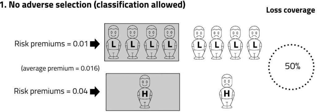
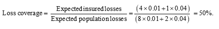
The weighted average of the premiums paid is (4 × 0.01 + 1 × 0.04)/5 = 0.016. Since higher and lower risks are insured in the same proportions as they exist in the population, there is no adverse selection. Exactly half of the population’s expected losses are compensated by insurance. I describe this as a ‘loss coverage” of 50%. The calculation is:
Next, consider Scenario 2. Risk classification has now been banned, so insurers have to charge a common pooled premium for all risks. High risks are more likely to buy, and low risks less likely (adverse selection). The shading denotes the three risks that are now covered. The pooled premium is set as the weighted average of the true risks, so that expected profits on low risks exactly offset expected losses on high risks. This weighted average premium is (1 × 0.01 + 2 × 0.04)/3 = 0.03.
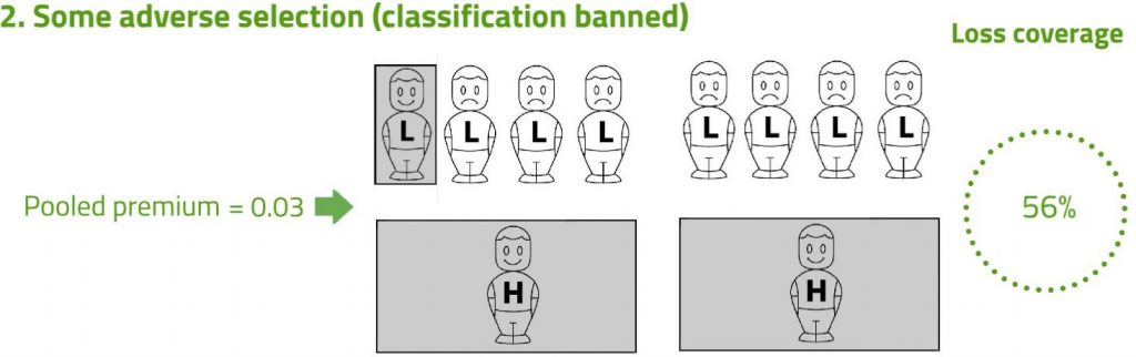
Note that in Scenario 2, the average premium paid is higher (0.03 compared with 0.016 before), and the number of risks covered is lower (three compared with five before). These are the essential features of adverse selection, which the example fully represents. But there is a surprise: despite the adverse selection, Scenario 2 achieves a higher expected compensation of losses.
Intuitively, this can be seen by comparing the shaded areas. In Scenario 1, the shading over one high risk has the same area as the shading over four low risks. Those equal areas represent equal quantities of risk transferred. Then notice that in Scenario 2, the total shaded area is larger than in Scenario 1. This represents more expected losses being compensated.
The visual intuition is confirmed when we calculate the loss coverage:
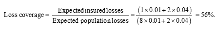
which is higher than the 50% in Scenario 1.
Scenario 2, with a higher expected fraction of the population’s losses compensated by insurance – higher loss coverage – seems to me superior from a social viewpoint to Scenario 1. The superiority of Scenario 2 arises not despite adverse selection, but because of adverse selection.
Another way of making the point is to say that that in Scenario 2 above, with some adverse selection, more risk is voluntarily traded than in Scenario 1. It seems odd that insurance economists describe an arrangement where more risk is voluntarily traded, and more losses are compensated, as “less efficient.”
So some adverse selection may be advantageous. But if it goes too far, this can lead to lower loss coverage. Scenario 3 illustrates this situation.
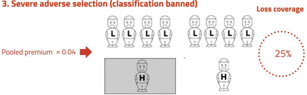
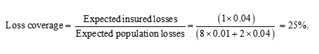
Adverse selection has now progressed to the point where no low risks, and only one high risk, buy insurance. The average premium paid is just the risk premium for the one high risk insured, that is 0.04. The shaded area is smaller than in both the earlier scenarios. The loss coverage is:
Taken together, the three scenarios suggest that risk classification increases loss coverage if it induces the ‘right amount’ of adverse selection (Scenario 2), but reduces loss coverage if it induces ‘too much’ adverse selection (Scenario 3). The argument is not sensitive to the particular numbers I have used; the point is quite general.
Which of Scenario 2 or Scenario 3 actually prevails depends on the response of higher and lower risks to changes in prices – that is, the demand elasticities of higher and lower risks. A number of papers (Thomas 2007, 2008, 2009, 2018; Hao et al 2016, 2018, 2019) and a book (Thomas 2017) look at this in greater detail. The broad-brush conclusion is that the argument is not just a theoretical curiosity; the elasticities required for restrictions on risk classification to give an increase in loss coverage seem realistic for many insurance markets.
In summary, from a public policy viewpoint, insurance works better with some adverse selection. The reasons, which were illustrated by the example, can be stated verbally as follows. Adverse selection involves a fall in total numbers insured, which is bad. But it also involves a shift in coverage towards higher risks, which is good. For modest degrees of adverse selection, the second effect will outweigh the first. Measuring efficiency by the number of individuals insured overlooks this trade-off between covering a large number of risks and covering the ‘right’ risks – the higher risks, the people who need insurance most.
2) Non-risk price discrimination
FH also consider individual price variations which do not reflect expected costs, described as non-risk price discrimination (the traditional economic term) or price optimization (the industry term). Non-risk price discrimination has been common practice in personal lines insurance for at least 15 years in Europe. It therefore seems remarkable that the topic has been almost completely ignored in both actuarial science and insurance economics literature. There are books on price and revenue optimization in general (Phillips, 2005) and a case study of price optimization from the perspective of a single insurer (Krikler et al, 2004). But neither of these consider the distinctive features of insurance (adverse selection, moral hazard, etc), or the public policy question of how non-risk price discrimination affects overall market outcomes.
My paper Thomas (2012a) which FH kindly cited made the following main points:
- Aggregate industry profits are likely to be increased where all insurers practise non-risk price discrimination against the same groups (best-response symmetry), but decreased where different insurers discriminate against different groups (best-response asymmetry).
- In particular, inertia pricing (i.e. higher mark-ups for renewing customers, compared with risk-equivalent new customers) is likely to reduce aggregate industry profits, because it involves best-response asymmetry: every insurer offers a discount to persuade the customers of other insurers to switch.
- Whilst inertia pricing may benefit customers in aggregate, not all customers are better off, and the distributional effects may be of concern to a regulator (e.g. the customers who do not switch regularly, and so are made worse off, are probably the less sophisticated or less informed). Furthermore, the high level of switching generated by inertia pricing is inefficient for society as a whole: it arises purely as an artefact of market structure, and does not reflect changing customer needs or preferences.
Whilst I thought these points were worth making, they were in the main a translation to the insurance context of standard concepts in the theory of price discrimination in general, which has origins going back a century (e.g. Pigou, 1920; Robinson, 1933). What was really needed was an integrated theory of these standard concepts with the distinctive features of insurance, such as risk-based pricing, adverse selection and moral hazard.
I originally envisaged pursuing the development of this integrated theory in subsequent papers. However, I found Thomas (2012a) difficult to publish – much more difficult than papers on other controversial topics such as ethical aspects of insurance discrimination (Moultrie & Thomas 1997), genetics and insurance (Thomas 2001, 2002, 2012b), and loss coverage (Thomas 2007, 2008, 2017, 2018). A succession of journal referees dismissed the relevance, or even the possibility, of non-risk price discrimination in insurance, with an indignation and vehemence that sometimes bordered on the absurd.
My impression was that these objections were not motivated by commercial considerations, but rather by intellectual and pedagogical anxieties. For many reasons outlined by FH, most new students beginning the study of insurance attach a negative connotation to the term “discrimination”. Insurance academics therefore spend a good deal of their time explaining that insurance discrimination is risk-based, that it increases the efficiency of insurance markets (not always, see section 1 above), that it should therefore not be assigned the negative connotation usually associated with discrimination, etc. But once it is admitted that much contemporary discrimination by insurers is in fact not risk-based, the argument becomes more complicated, and the questionable foundations of what insurance academics think they know are exposed. Perhaps the truth is too messy to contemplate, and too disreputable to teach. It was certainly difficult to publish, or at least it was in 2012; and so I reluctantly concluded that pursuing the topic further would not be a good use of time, at least from a personal perspective.
As FH note, non-risk price discrimination is a topic of active regulatory interest and intervention in some jurisdictions. The United Kingdom regulator banned higher pricing for insurance renewals compared with risk-identical new customers with effect from 1 January 2022 (Financial Conduct Authority, 2020, 2021). Apart from Thomas (2012a) – which as noted above, actually suggested there might be some merits to inertia pricing – there were no academic studies which could inform this decision either way. I know this because the regulator contacted me to ask if I knew of any further studies. As far as I am aware, the position is similar in other jurisdictions, and it seems to me a striking failure of the academic community. By considering the topic, FH have a step towards rectifying this omission. So I congratulate them once again for this, and for the other contributions of their paper.
(END of full comment submitted to NAAJ)
APPENDIX: The statistical fairness trilemma
Here is the standard “confusion matrix” for a binary predictor (stated in the context of medicine but it could just as well be high/low risk). D and D across the top are disease and no disease, T and T along the side are test positive and test negative. The four cells contain counts of cases, and so classify the entire population by disease status and test result.
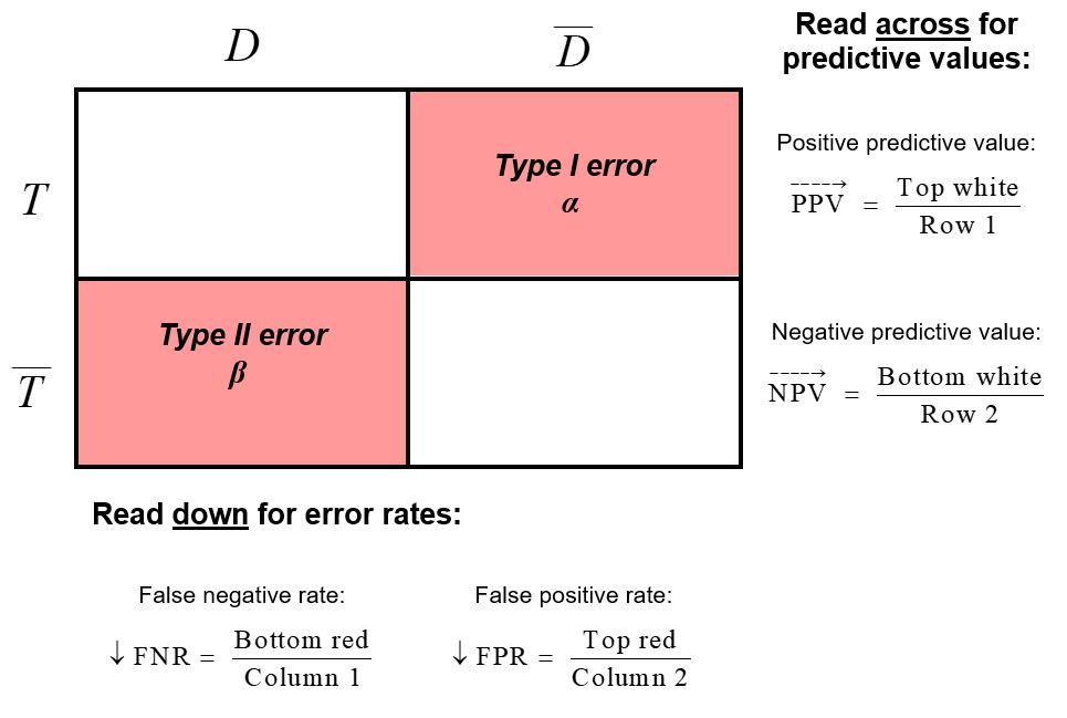
Now let p be the base rate (true probability of disease in the population). The true odds p/(1-p) are given by Column 1 / Column 2. We then have the identity:
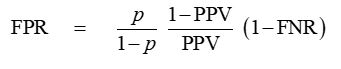
which is easy to verify using the definitions shown in the diagram. Then think about what happens when we move from one population to another with a different base rate p:
- The ratio of the columns will change.
- “Well-calibrated” implies that the ratio of the rows must change in same proportion.
- But for FPR and FNR to be the same across the two populations, the identity requires that PPV/(1-PPV) must also change in same proportion as p/(1-p).
- But PPV/(1-PPV) is Top white / Top red …
… In general, this is not going to work: we have too many constraints on the columns and rows and cells. One exception: where the red error cells are empty for both groups (i.e. the identity collapses to 0, and we have a perfect predictor).
It is however always possible, in principle, to satisfy any two of the three constraints in the trilemma. For example, well-calibrated + equal false positive rates:
- This gives, for each group, a constraint on the ratio of the rows, and a constraint on (Top red / Column 2).
- We can satisfy these simultaneously by adjusting our predictor to shift cases between the two cells in Column 1.
- But this will inevitably violate the third constraint, equal false negative rates.
I said “in principle” because the shift of cases between cells at the second step was idiosyncratic. In practice, it may be difficult to find a predictor which exactly achieves this; but in principle, it is possible.
I note that the verbal descriptions can vary, e.g. Cathy O’ Neil’s blog commentary on her toy example linked above defines the “false positive rate” as (Top red / Row 1). But the underlying idea applies whatever the descriptions: “too many constraints on the columns and rows and cells”.
Finally, an alternative way of writing the key identity is
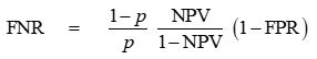
which references the constraints via the second row (i.e. NPV) rather than the first (i.e. PPV).